


Let’s start with a familiar example: sitting down to write an article. You’ve got an idea, you’ve got a basic structure, you might even have a deadline. You start writing. The next day you might well be writing some more, you might be editing, you might be completely distracted by something else entirely. A bit of research becomes a whole lot of research. Before you know it you’ve got seventeen browser tabs open, three potential titles, and absolutely nothing at all.
Now what if we could actually describe this very erratic process in mathematical terms? What if we could work out the probability of being productive tomorrow given what we’re doing today?
This is where Markov chains become interesting.
A Markov chain is a mathematical model for a system that evolves from one state to another over time. Given the current state, the past is irrelevant in terms of predicting the next state. That’s the Markov property.
In this article, we’re going to look at Markov chains using a small fictional writing exercise example. We’ll look at transition matrices, work out multi-step probabilities, look at stationary distributions and then go on to actually implement a Markov chain in Python.
We’ll also talk about something I think deserves a bit more attention: just because we can model something as a Markov chain doesn’t mean we necessarily should.
1. The Writing Experiment: Three States, Many Possibilities
Let’s imagine a writer working on an article over several days. Each day, we classify their activity into one of three mutually exclusive states:
-
Drafting (D): Actively writing new material.
-
Revising (R): Editing and improving existing material.
-
Distracted (X): Doing practically everything except working on the article.
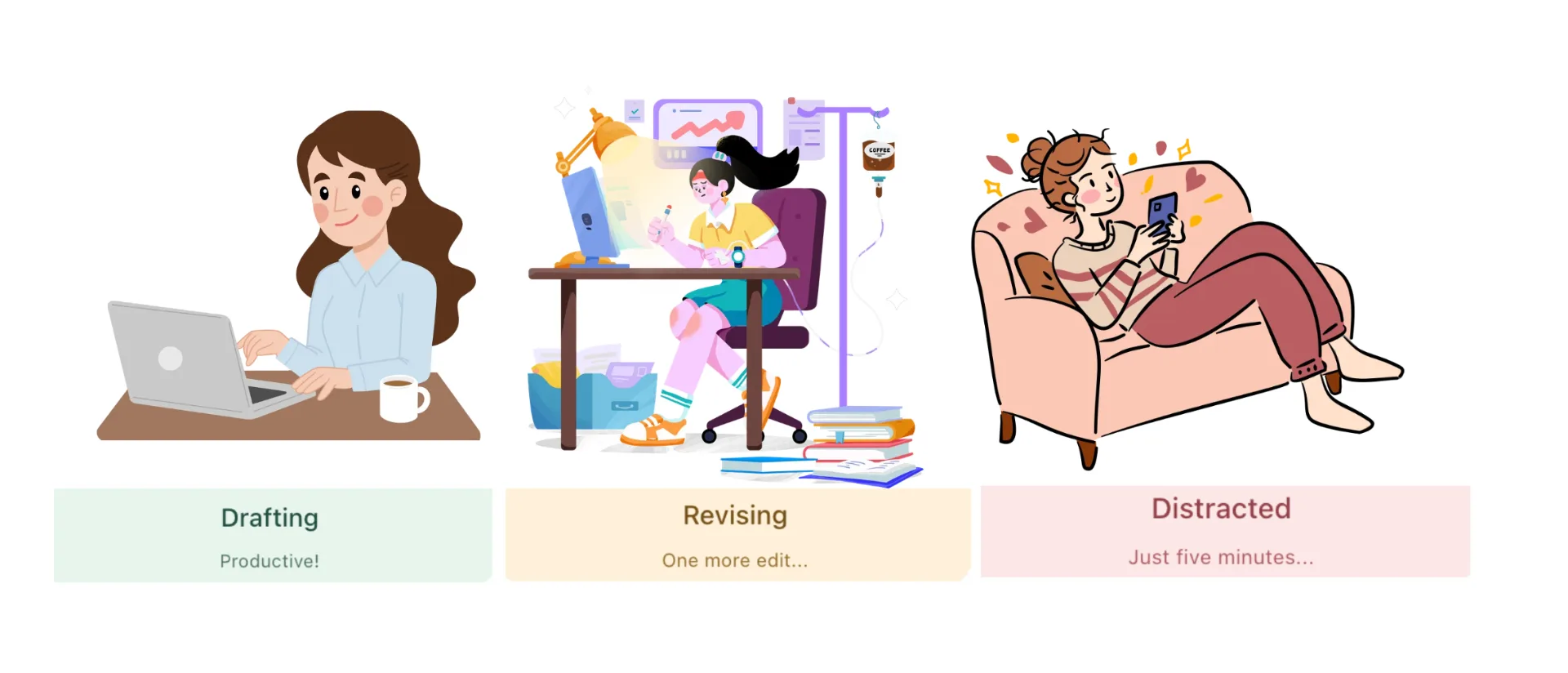
To keep the example manageable, suppose we observe one state per day, representing the writer’s primary activity. Now imagine we have estimated the following transition probabilities:
Let’s interpret the first row of the table. If the writer is drafting today, there’s a 60% chance they’ll continue drafting tomorrow, a 30% chance they’ll move to revising, and a 10% chance they’ll become distracted. Interestingly, if they are distracted today, there’s still a 60% combined chance of coming back to drafting or revising tomorrow. Procrastination may not be quite as permanent as we sometimes think.
The key point is that we’ve described the writer’s behavior in terms of states and the probabilities of transitioning between those states. That’s the basis of a Markov chain.
2. The Markov Property: Does Yesterday Really Not Matter?
The defining feature of a first-order Markov chain is its memoryless property.
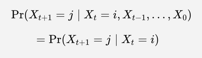
Here, (X_t) represents the state of the process at time (t), while (i) and (j) represent possible states.
Don’t worry if the notation looks intimidating. The idea is simpler than it appears.
Suppose our writer is drafting today. According to the transition probabilities, the probability that they’ll be revising tomorrow is 30%. But what if they were distracted yesterday? Still 30%.
And what if they have been drafting for the past five days? Again, 30%.
So, essentially, once we know today’s state, the model does not use the previous states to determine tomorrow’s probabilities.
However, an assumption that appears reasonable may not be so in reality. A writer who has been distracted for five consecutive days may behave differently from someone who has been steadily making progress.
The Markov property simply assumes that today’s state summarizes everything from the past that is relevant for predicting the next state. Whether this assumption is reasonable depends on the system we’re modeling and how we’ve defined our states.
We’ll return to this question later.
3. Understanding the Transition Probability Matrix
We can represent our three-state system using a transition probability matrix:
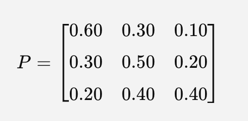
The rows and columns follow the order Drafting, Revising, Distracted. Each element represents the probability of moving from one state to another in one time step. For example, the element in the first row and second column is 0.30. This represents the probability of moving from Drafting to Revising.
There are two important rules for a valid transition matrix:
First, every element must lie between 0 and 1.Probabilities cannot be negative or greater than one.
Second, the elements in each row must sum to one.For instance, the first row gives: 0.60+0.30+0.10=1
After all, tomorrow the writer must be in one of the three states we’ve defined. A matrix satisfying these conditions is called a row-stochastic matrix. Once we have prepared this matrix, we can start answering more intriguing questions.
Suppose our writer is drafting today. We know there’s a 30% probability that they’ll be revising tomorrow. But what is the probability that they’ll be revising two days from now?
There are three possible ways this could happen.
Path 1: Drafting → Drafting → Revising
The writer continues drafting tomorrow and moves to revising the following day.
Probability: 0.60 * 0.30 = 0.18
Path 2: Drafting → Revising → Revising
The writer switches to revising tomorrow and continues revising.
Probability: 0.30 * 0.50 = 0.15
Path 3: Drafting → Distracted → Revising
The writer gets distracted tomorrow but returns to revising the following day.
These paths are mutually exclusive, so we can add their probabilities.
Therefore, the probability of being in the Revising state two days from now, starting from Drafting, is 0.18+0.15+0.04 = 0.37 or 37%
This calculation illustrates the Chapman–Kolmogorov equation.For a time-homogeneous Markov chain:
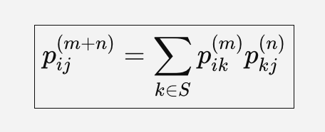
It tells us that the probability of moving between two states over multiple steps can be calculated by considering all possible intermediate states. Thankfully, we don’t need to manually enumerate every path. Matrix multiplication does exactly this.
For our example, the two-step transition matrix can be written like this.
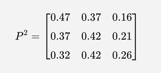
The first row represents the probabilities two days into the future, conditional on being in the Drafting state today. For a time-homogeneous Markov chain, the (n)-step transition matrix is:
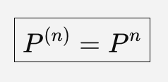
This is what makes Markov chains computationally convenient. Once the transition matrix is specified, we can calculate future state probabilities without individually tracking every possible path.
5. Stationary Distribution: Will We Eventually Find a Pattern?
Here’s another interesting question. What happens if the writer just keeps toggling between those three states for a very long time? Do the probabilities go on changing forever? Or do they eventually settle down?
For our example, the probabilities converge to a stable distribution, which is known as the stationary distribution.
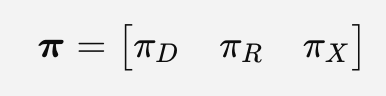
The stationary distribution satisfies:
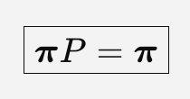
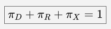
Solving these equations for our transition matrix gives:
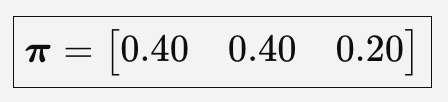
What does this mean? In the long run, the writer’s state probabilities approach:
Under the standard ergodicity conditions, these are also the long-term proportions of time spent in each state. Our hypothetical writer is therefore spending around 80% of their days actually writing (i.e. drafting or revising).
However, we need to be clear that a stationary distribution does not mean the system has stopped changing states. It just means that the probability distribution remains unchanged.
The writer may still go from Drafting to Distracted, Distracted to Revising and back again to Drafting. The individual outcomes remain random. The overall distribution does stabilize.
Also, we shouldn’t assume that every Markov chain will converge to its stationary distribution. Some are periodic, some have multiple communicating classes and some have absorbing states.
6. Let’s Build Our Markov Chain in Python
Let’s move from equations to implementation. We’ll use NumPy for the calculations and Matplotlib to visualize how the probability distribution changes over time.
First, define our transition matrix.
import numpy as npimport matplotlib.pyplot as pltstates = ["Drafting", "Revising", "Distracted"]P = np.array([[0.60, 0.30, 0.10],[0.30, 0.50, 0.20],[0.20, 0.40, 0.40]])# Validate the transition matrixassert np.all(P >= 0)assert np.all(P <= 1)assert np.allclose(P.sum(axis=1), 1)Calculating the Two-Step Transition Matrix
P2 = np.linalg.matrix_power(P, 2)print(np.round(P2, 2))[[0.47 0.37 0.16][0.37 0.42 0.21][0.32 0.42 0.26]]Again, we can see that the probability of moving from Drafting to Revising over two days is 0.37.
Forecasting the Next 20 Days
Now assume our writer is definitely drafting today.
Let’s calculate the probability distribution for the next 20 days.
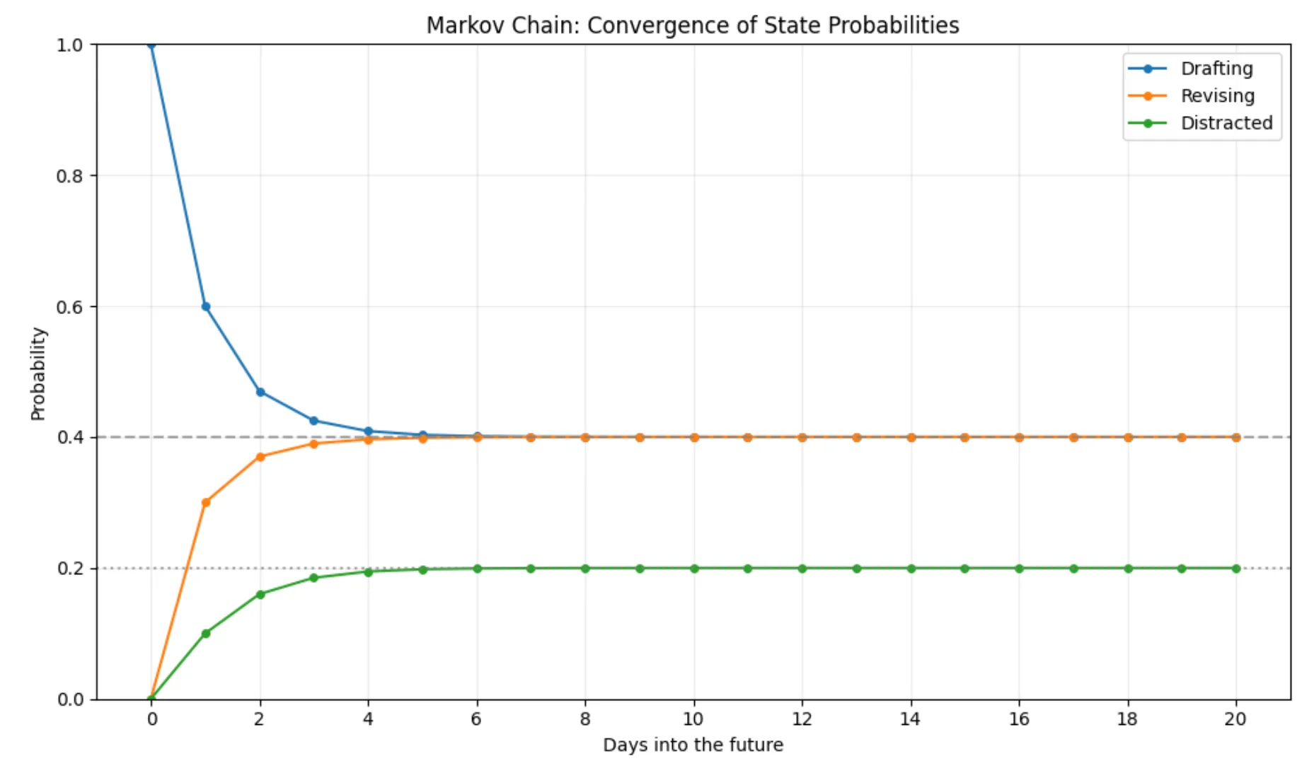
initial = np.array([1.0, 0.0, 0.0])days = np.arange(21)probabilities = np.array([initial @ np.linalg.matrix_power(P, int(n))for n in days])print("Day 20 probabilities:")for state, prob in zip(states, probabilities[-1]):print(f"{state}: {prob:.4f}")The probabilities approach 0.40, 0.40, and 0.20. Now, let’s visualize the convergence.
plt.figure(figsize=(10, 6))for i, state in enumerate(states):plt.plot(days,probabilities[:, i],marker="o",markersize=4,label=state)plt.axhline(0.40, color="gray",linestyle="--", alpha=0.7)plt.axhline(0.20, color="gray",linestyle=":", alpha=0.7)plt.xlabel("Days into the future")plt.ylabel("Probability")plt.title("Markov Chain: Convergence of State Probabilities")plt.xticks(days[::2])plt.ylim(0, 1)plt.legend()plt.grid(alpha=0.25)plt.tight_layout()plt.show()The resulting plot shows the initial probability of Drafting gradually decreasing while the probabilities of Revising and Distracted increase. Eventually, the state probabilities stabilize.
Simulating a Single Writing Journey
I want to demonstrate one more distinction. The probabilities approaching 40%, 40%, and 20% don’t mean every sequence of ten days will contain exactly four drafting days, four revising days, and two distracted days. Let’s simulate one possible sequence.
rng = np.random.default_rng(42)current_state = 0 # Draftingpath = [current_state]for _ in range(29):current_state = rng.choice(len(states),p=P[current_state])path.append(current_state)print(" → ".join(states[i] for i in path))The result is one randomly generated 30-day trajectory. Run the simulation with different random seeds and you’ll obtain different sequences. This is the difference between the theoretical probability distribution and an individual realization of the stochastic process.
7. Important Properties of Markov Chains
Now that we’ve built a working example, let’s explore the properties that determine how a Markov chain behaves.
7.1 Time Homogeneity
Our example assumes that transition probabilities remain constant over time. The probability of moving from Drafting to Revising is always 30%, regardless of which day we’re considering.
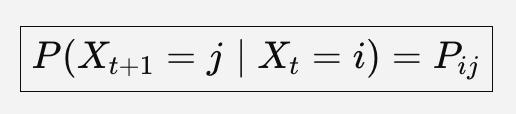
The right-hand side is time-independent. That’s a time-homogeneous chain. Now imagine a writer facing a very tight publication deadline. As the deadline draws nearer the probability of moving from Distracted to Drafting could well increase dramatically. The transition probabilities would then be time dependent. Importantly, a time-inhomogeneous chain can still be Markov. Time homogeneity and memorylessness are two different assumptions.
7.2 Irreducibility
A Markov chain is irreducible if every state can eventually be reached from every other state with positive probability. In our example, a writer can transition between Drafting, Revising, and Distracted. There are no permanently inaccessible states. Therefore, our chain is irreducible. This matters because irreducibility helps establish whether the chain has a unique stationary distribution.
7.3 Aperiodicity
A Markov chain is periodic when its states can only be revisited at time intervals following a fixed cycle. For example, suppose a simplified system alternates deterministically between two states:
A → B → A → B → A.
Starting from A, we can only return to A after an even number of steps. Its period is 2.
This chain can have a stationary distribution without its probability distribution converging from a fixed starting state. Our writing example is different. The writer has a positive probability of remaining in the same state on the next day. This makes the chain aperiodic.
For a finite-state Markov chain, irreducibility and aperiodicity together guarantee convergence to a unique stationary distribution.
7.4 Absorbing States
An absorbing state is one that cannot be exited once entered. Suppose we extend our writing example by adding a fourth state: Published.
If we define Published as the completion of this particular writing project, there is no transition back to the earlier states within that project.

The Published state is absorbing. Such models are useful when studying processes that have a well-defined terminal event. Examples include an insurance claim reaching final settlement, a component permanently failing, or a customer permanently exiting a particular service. However, an absorbing chain behaves differently from our original irreducible three-state model.
Once absorption becomes possible, the long-run distribution can be dominated by absorbing states. So we shouldn’t automatically apply our earlier 40%–40%–20% stationary distribution to the expanded model.
8. But What If Yesterday Actually Matters?
So far, we’ve assumed that knowing today’s state is sufficient to predict tomorrow.
Let’s challenge that assumption. Imagine we collect actual observations of the writer’s activity and estimate the following probabilities.
These are hypothetical values for a separate experiment. Note that the current state is the same in both cases: Drafting.
Yet the chance of drafting tomorrow is contingent on yesterday’s state. A person who’s been drafting all day is far more likely to be drafting tomorrow than someone who has only just got back into it after a distracted day. If this difference is real and not just sampling variation then our first-order Markov assumption is inadequate.

In this situation, we might consider a second-order Markov model:
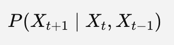
Now the next state depends on the previous two states. Alternatively, we could redefine the states to preserve more information about recent behavior.
For example, instead of simply describing someone as Drafting, we could distinguish between:
This makes the state space larger but potentially more informative.
A Markov model doesn’t have to ignore history completely. It needs a state representation that adequately summarizes the relevant history.
This is why choosing states is often more difficult than performing the calculations. A transition matrix may be mathematically valid while still failing to capture important aspects of the underlying process.
9. Where Do Markov Chains Become Useful in Practice?
Our example involved writing an article, but the mathematics applies to many real-world problems.
In credit risk, transition matrices can describe the movement of borrowers between credit rating categories. They can be used to estimate multi-period rating migration and default probabilities under suitable assumptions.
In customer analytics, states might represent active, inactive, and churned customers. Markov models can help describe customer movement between engagement categories.
In reliability engineering, a machine might transition between working, degraded, and failed states.
In web analytics, states can represent different pages or stages of a user journey.
In natural language processing, classical Markov-based models describe sequence transitions, although modern language models use substantially more complex architectures.
The same fundamental principle underpins all of these applications: model the system in terms of states, estimate the transition probabilities and then look at how the system evolves.
But the appropriate state definitions, time intervals, and model assumptions vary considerably. For instance, in credit-risk modeling, transition probabilities may depend on economic conditions. A matrix estimated during a stable period might not adequately describe rating migrations during a recession. A possible extension is to estimate different transition matrices conditional on economic regimes. This introduces additional complexity, but it may also produce more realistic forecasts.
10. What Markov Chains Can and Cannot Tell Us
There’s one final caveat to mention. Our writing model can work out the probability of being in Drafting, Revising or Distracted at some future point. But can it tell us when the article will, in fact, be published? Maybe not with the current state definitions.
There’s no completion event in our three-state model. To answer that question you’d have to modify the model in some way (perhaps by introducing an absorbing Published state and specifying the transition probabilities into it). That’s a general modeling lesson.
The questions the model can answer are going to be a function of how we’ve defined its state space. A Markov chain may be easy to calculate, but that simplicity in no way removes the need for careful modeling decisions.
We still need to consider the relevance of the past observations, the stability of the transition probabilities, the completeness of our state definitions and whether the model is in fact doing a good job on data it has never seen.
Final Thoughts
Markov chains offer an elegant way to understand systems that evolve probabilistically over time.
With a relatively simple transition matrix, we can calculate future state probabilities, study long-run behavior, and explore the conditions under which a system converges to a stationary distribution.
But the most important part of a Markov chain isn’t matrix multiplication. It is the assumption about what the present state tells us about the future.
The Markov property is of course very powerful in that it allows us to turn a very complicated history into something that is manageable. The difficulty is knowing when that is a reasonable thing to do. Our hypothetical writer may have spent the entire week procrastinating. The math may well choose to ignore that history. Whether or not tomorrow is going to be just as lenient is another matter entirely.
-
J. R. Norris, Markov Chains, Cambridge University Press.
-
Sheldon M. Ross, Introduction to Probability Models.
