Timestral, t0, Tabby, and Morpheus-2.0 Compared on GIFT

Imagine forecasting tomorrow’s hourly electricity demand at a substation. You have the last week of load readings (168 numbers) and tomorrow’s temperature forecast. A traditional approach would fit a model to that substation’s history. A foundation model takes another route: a model trained on other series produces the forecast, uncertainty bands included, without being fitted to that substation at all.

Between 10 September and 16 October 2026, four organisations released models pursuing that goal: Huawei’sTabby, The Forecasting Company’s (TFC’s)t0-gamma, Mistral’sTimestral, and JPMorganChase’sMorpheus-2.0. Their close release dates make for a useful comparison of how different teams approach the same problem.

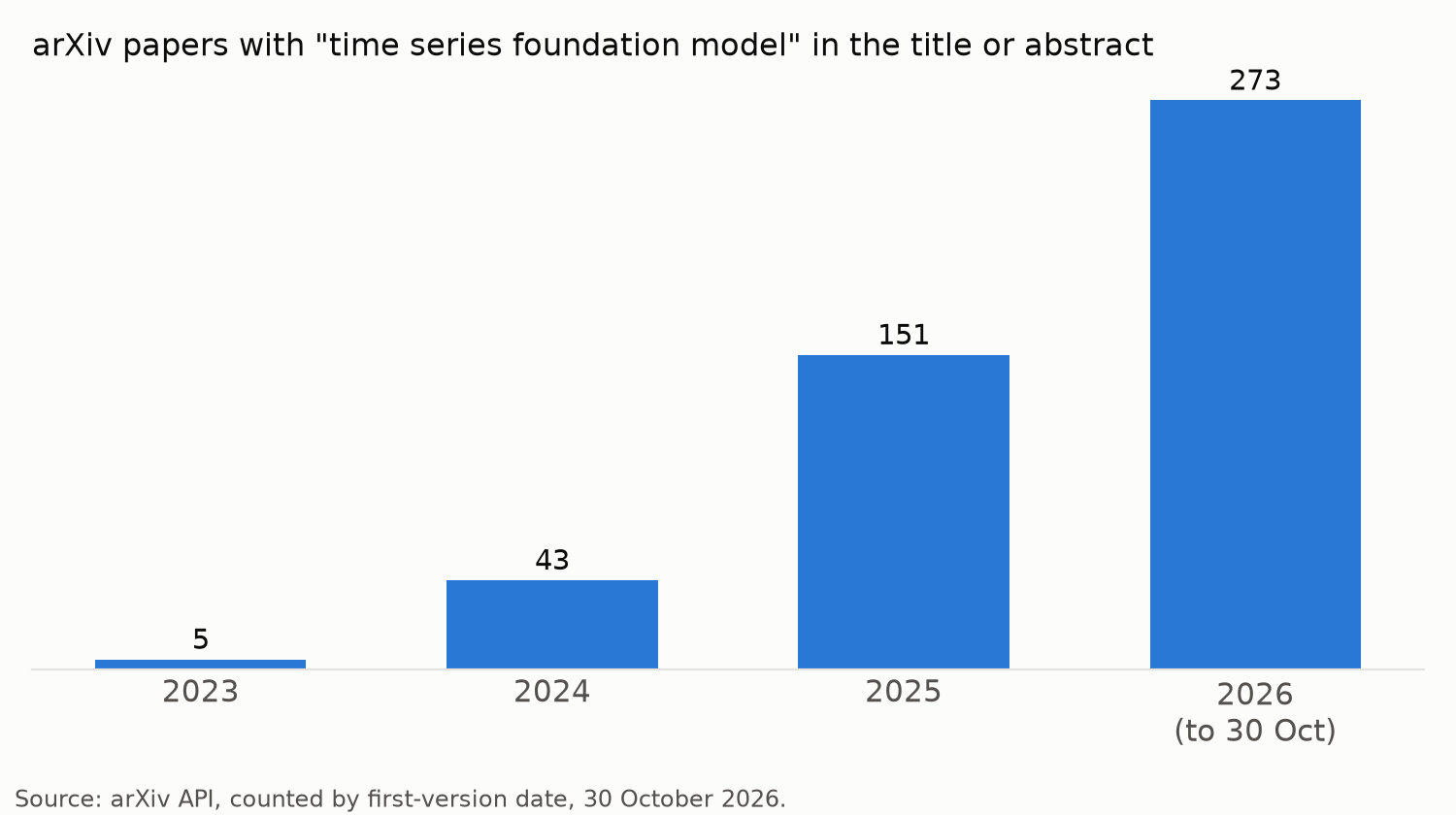
The field has grown quickly. In 2023, five arXiv papers mentioned “time series foundation model” in their title or abstract; the count rose to 43 in 2024, 151 in 2025 and 273 by 30 October 2026 (arXiv search, counted by first-version date). Use has grown alongside research: Amazon’s Chronos-2 was downloaded 11 million times from Hugging Face in the 30 days to 30 October.

Earlier this year I reproduced t0-alpha’s benchmark score exactly. This time I examined the four architectures, compared their published scores on the same tasks, measured how much t0-gamma benefits from inference-time adjustments and reran the three models with public weights. I wanted to know what explains the gains and which differences matter for a real forecasting problem.

Takeaways

• A common recipe has emerged. All four scale numerical inputs, divide them into patches, process them with transformers and predict quantiles. Synthetic data plays a major role in training.

• The important architectural difference is how series communicate. Tabby forecasts each series independently. Timestral and t0 exchange information between series in selected layers; Morpheus does so in every layer. That matters when temperature, promotions or other known drivers could improve a forecast.

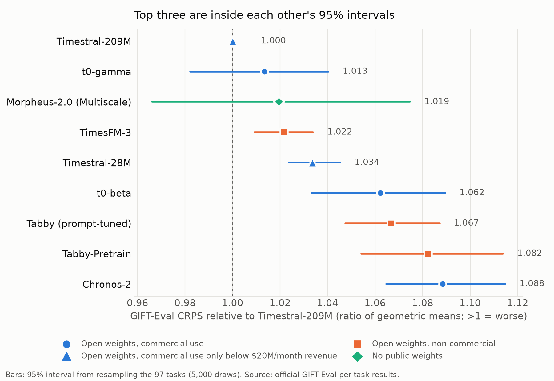
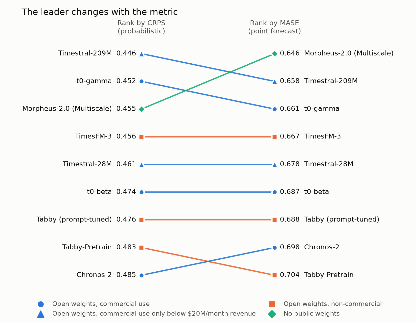
• The top three are difficult to separate on aggregate GIFT-Eval scores. Timestral leads on probabilistic CRPS, Morpheus on point-forecast MASE, and pairwise confidence intervals include a tie.

• Training appears to explain much of the recent improvement. t0-gamma’s inference-time adjustments explain less than a tenth of its gain over t0-beta. Morpheus’s ablations and Tabby’s authors also point to data and training.

• Deployment constraints matter. Licence, access to weights, support for covariates and results on your own data can outweigh small leaderboard differences.

A foundation model replaces fitting a model for each series

Traditionally, we might fit ARIMA or exponential smoothing to the substation’s historical readings, capturing daily and weekly patterns and tuning parameters to that location. This can work well with enough history. Across 10,000 substations, however, fitting, monitoring and updating separate models becomes expensive. A newly installed substation may have too little history for reliable local fitting.

A time-series foundation model is pretrained on many other series. At prediction time it reads the substation’s recent history and produces a forecast in a forward pass, without updating its weights for that substation. This is zero-shot forecasting. The analogy is to a language model handling a new piece of text without being retrained on that document.

There is a difference between words and time-series values. Language models process tokens from a vocabulary; numerical series can range from fractions of a degree to millions of website requests. The shared forecasting recipe starts by making those numbers manageable.

Scaling. Each model subtracts a mean, divides by a standard deviation and applies the inverse hyperbolic sine, or asinh. Near zero, asinh behaves approximately like a straight line; at large magnitudes it compresses values somewhat like a logarithm. That helps a model handle both megawatt readings and web-traffic counts without a single spike dominating. Timestral and t0 calculate their statistics causally, using only values available up to each point, so later observations cannot influence the scaling of earlier ones.

Patching. Instead of feeding 168 separate hourly readings into the transformer, the model groups consecutive values into short blocks called patches. Each patch becomes one token, much as a language model groups characters into text tokens. Timestral and t0 use 32-step patches: 168 hours are padded to 192 and represented by six tokens. Tabby uses 16-step patches; Morpheus uses four. Tokens also carry missing-value masks so a sensor outage is not mistaken for a real zero. Longer patches reduce token count and attention cost, but may cut across patterns such as a 24-hour daily cycle.

The transformer. Tokens pass through between 9 and 24 transformer layers. In each layer, attention lets every token weigh how relevant the other tokens are and take a weighted average of their information. This is where the models differ most: some layers read only the history of one series, while others allow information to pass between related series.

Quantile outputs. The output is a set of quantiles, for example tomorrow’s 6pm load at the 10th, 50th and 90th percentiles. The median gives a point forecast; the outer quantiles describe uncertainty. Timestral, t0 and Morpheus output 21 levels; Tabby outputs 99. Timestral, t0 and Tabby enforce non-crossing quantiles by predicting one level and adding positive increments. Morpheus predicts them separately, allowing crossing.

Synthetic training data. All four use substantial generated data. Public real-world series are limited, and some overlap with forecasting benchmarks. Synthetic series add variety while reducing the risk of training on test windows. Each lab has built its own generator, discussed below.

This recipe was not inevitable. Amazon’s original Chronos (2024) discretised values into bins, and Salesforce’s Moirai predicted a mixture of distributions. Chronos-Bolt and Chronos-2 later adopted patches; Moirai 2.0moved to quantile outputs and attributed much of its gain to the backbone and output design. All nine 2025–26 models I compared use patches and quantile outputs: Chronos-2, TimesFM-3, Moirai 2.0, Toto 2.0, TiRex-2 and the four here.

The first difference: which series a model can read

Return to the substation. Demand is one series; temperature is another. If tomorrow will be unusually hot, the temperature forecast might help predict air-conditioning demand. But a model can use that information only if its load-forecast tokens are allowed to read the temperature tokens.

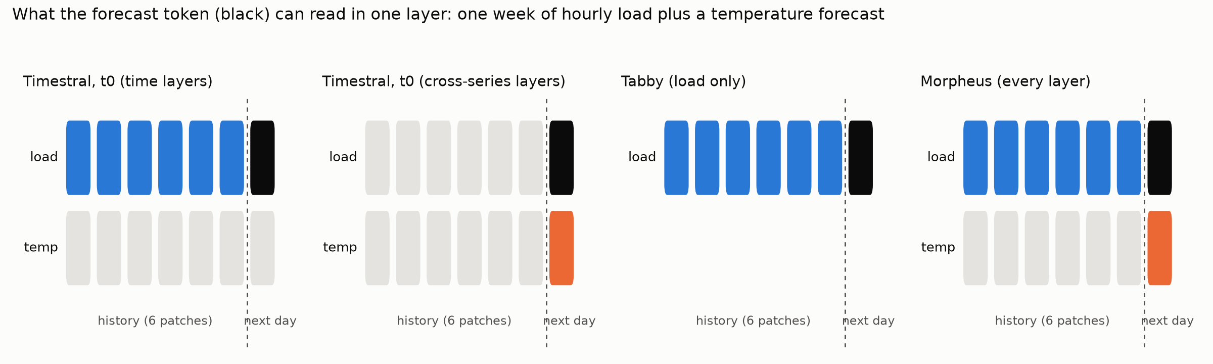
Tabby: one series at a time. Tabby is channel-independent: it splits multivariate inputs into individual series and forecasts each independently. It predicts load from past load, without tomorrow’s temperature. This is simple, with cost growing linearly with the number of series, but sacrifices potentially useful drivers. On a hot day it must infer any likely demand spike from the load pattern alone.

Timestral and t0: exchange information in selected layers. Most layers attend across time within a series. In a cross-series layer, a token can read other series at the same time position. Timestral-209M has 24 layers; every fourth layer adds cross-series attention after time attention (six of 24). t0-gamma also has 24 layers, but every third layer is a cross-series layer instead of a time layer (eight of 24). Both control the direction of information flow: a target may read a known covariate (a driver whose future values are known in advance, such as a temperature forecast), but a covariate cannot read future target values. This avoids leaking tomorrow’s answer into the forecast. The pattern draws on Amazon’s Chronos-2; t0’s code credits Chronos-2 for cross-series attention and Datadog’s Toto for its backbone.

Morpheus-2.0: both axes in every layer. Morpheus arranges tokens on a grid of variables by time. Each of its nine layers runs attention along time and across variables at the same time step, then mixes the two with a learned weight. Full attention over every variable-time token would require memory growing quadratically with the combined grid size. Restricting attention to the two axes is cheaper; the paper reports that peak memory falls by more than half. In the paper’s ablations of the single 81.5M model, the full design scores 0.685 MASE (the leaderboard entry is a larger ensemble, covered below); fixing the mixture at 50/50 raises error to 0.725; replacing the two-axis design with full attention raises it to 0.759.

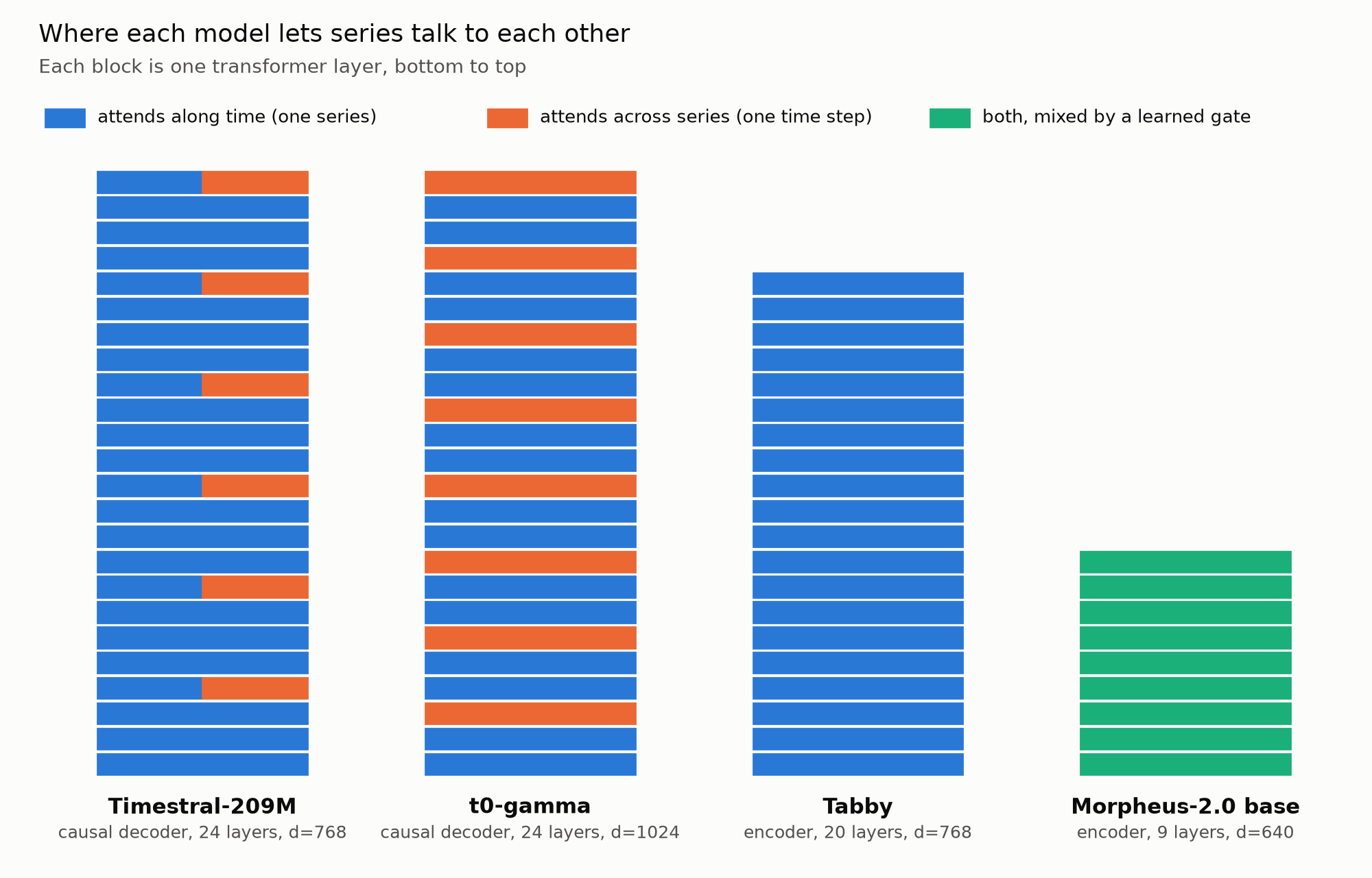
These are three ways of paying for information. Tabby avoids cross-series attention and cannot use the temperature forecast. Timestral and t0 spend some layers on it. Morpheus spends every layer but restricts attention to control memory. Whether the extra computation pays off depends on the data, particularly whether the covariates carry information the target’s own history lacks.

The second difference: how the forecast is produced

After reading the history, the model still has to produce the next 24 hourly values. The four releases use three approaches.

Timestral adds forecast tokens. Timestral appends learned future tokens after the history. History tokens read only earlier history; each forecast token reads the history and predicts 32 steps of quantiles. Up to 32 forecast tokens fit in one pass, giving 1,024 steps. Our 24-hour forecast needs one token. Mistral argues that this leaves the history representation intact rather than overwriting it with future placeholders.

t0 predicts the next patch. Like a next-token language model, t0 trains each patch to predict the following one. At forecasting time the future is represented by blank patches, and the last history patch predicts the first 32 future values. Up to 1,024 steps emerge in one pass. Training and inference use the same next-patch task, but information moves only forwards through the sequence. For a one-day forecast, Timestral and t0 both answer in a single pass; the difference is whether dedicated learned tokens or the history’s own last patch carry the prediction.

Tabby and Morpheus fill masked future positions. These are encoders, closer in spirit to BERT than GPT. Future values appear as masked positions; attention operates over the permitted context, and the model fills the future in one pass. Tabby uses a fixed 8,192-step window. The 168 history values and 24 future positions sit at the right-hand end, with roughly 8,000 padded steps in front; padding is excluded from attention. This is straightforward but caps its context at 8,192 steps.

For horizons longer than one pass covers (1,024 steps for Timestral and t0), Timestral, t0 and Morpheus extend forecasts by feeding the predicted median back as if observed. This is convenient but discards uncertainty from the previous pass, so intervals for very long horizons may be too narrow.

Four models, four training strategies

The architectures explain what each model can read. Training helps explain what it has learned to do with that information.

Timestral (Mistral, 15 October 2026)

Timestral comes in four sizes, from 5M to 209M parameters, and supports contexts of up to 32,768 steps, the longest of these releases. Mistral describes mostly synthetic training data: individual series with trends, seasonality and noise are combined into multivariate examples with nonlinear dependencies. Pretraining uses synthetic data at an 8,192-step context; a later stage mixes real and synthetic data at four times that length. Mistral had not published a technical report by 30 October 2026.

Its default forecaster also predicts the negated input series, flips that prediction back and averages the two. This makes the forecast more symmetric to upward and downward movements at the price of a second forward pass. It clips forecasts at zero when the history never goes negative. Mistral reports 17 milliseconds for a one-day forecast using the 5M model on eight CPU threads and 113 milliseconds for 209M; the 28M model is reported as 3.6 times faster than 209M, or about 31 milliseconds.

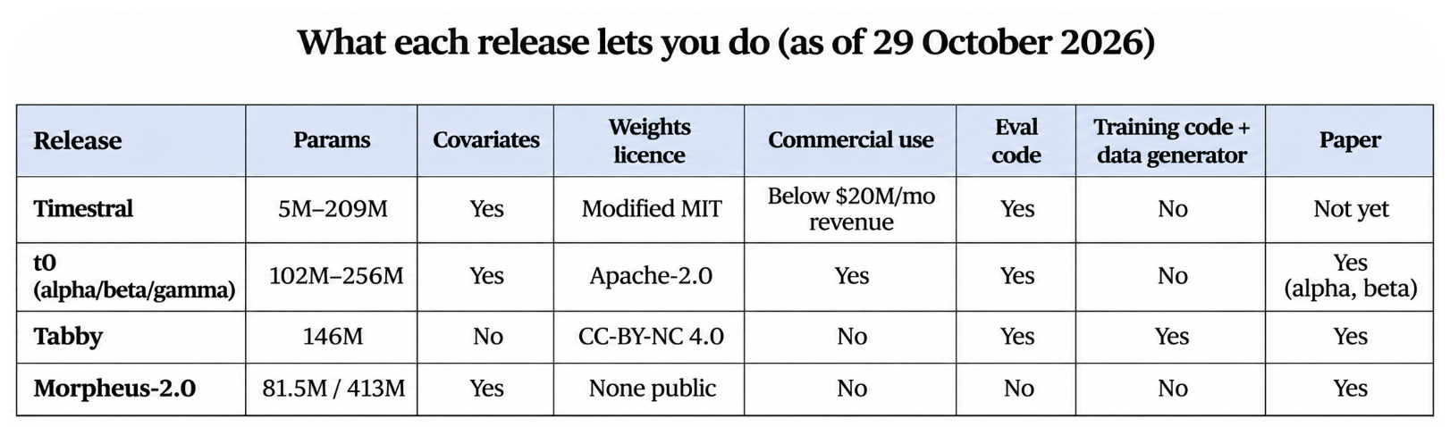
The inference code is Apache-2.0. The weights use a modified MIT licence: a company with more than $20 million in monthly revenue receives no rights without purchasing a commercial licence.

t0 (The Forecasting Company, June–October 2026)

t0-alpha has 102M parameters; beta and gamma each have 256M. All three are Apache-2.0. The t0 paperdescribes alpha’s training on GIFT-Eval’s public pretraining collection plus four synthetic families, including one million series generated from random cause-and-effect graphs. Training took 28 hours on four H100 GPUs.

Each patch token carries a learned role label: target, past-only covariate or known-future covariate. This tells the network which information is available at prediction time. Beta and gamma have identical architectures. TFC has not publicly explained what changed in gamma’s training, an important limitation when interpreting its improved score. It distributes ONNX, Apple-silicon and DuckDB runtimes; DuckDB can generate a forecast inside a database query.

Tabby (Huawei Noah’s Ark Lab, Paris, September 2026)

Tabby is a 146M-parameter, 20-layer encoder. Its paper emphasises training data and procedure rather than a new architecture. Its CauKerV2 generator draws base signals from ten families, including spikes, trends, random walks and chaotic systems, and connects them with random cause-and-effect graphs. The generated series therefore depend on one another through those graphs.

Training applies quantile loss at intermediate layers as well as the last, encouraging earlier layers to learn useful forecasts. It also restarts the learning-rate schedule three times, producing checkpoints along the way.

The base zero-shot model is Tabby-Pretrain. The leaderboard’s Tabby entry adds 160 learned prompt vectors, about 0.9M extra parameters, ahead of the frozen base model. Those vectors were trained on 48 GIFT-Eval training tasks, analogous to prompt tuning in language models. Huawei released the generators, training code and pipeline in its huawei-noah/trustworthyAI repository. The weights are CC-BY-NC 4.0, ruling out commercial use under that licence.

Morpheus-2.0 (JPMorganChase, 16 October 2026)

Morpheus-2.0 is an 81.5M-parameter, nine-layer encoder using two-axis attention. Its synthetic MySTiC dataset contains 22 billion observations, including targets driven by known variables through delayed or nonlinear relationships, alongside irrelevant distractor series. The design is meant to teach cross-series attention to use the drivers and ignore the distractors.

Its training ablations show how much data and curriculum matter. The full model, trained with MySTiC and a four-stage curriculum moving from synthetic to mostly real data, scores 0.685 MASE. Without the curriculum it scores 0.759 (by coincidence the same figure as the full-attention ablation); trained on real data alone, 0.814. Training used one node of eight A100 GPUs.

Its Multiscale variant combines five encoders with different patch lengths and a learned mixing head that weights their forecasts per series. The paper refers to “released checkpoints”, but I found no public weights or code on Hugging Face, GitHub or in the paper as of 29 October 2026. That limits independent reproduction. This 413M-parameter ensemble, not the single model, is the one on the leaderboard.

What looks settled, and what remains open

Patching and quantile outputs have become common design choices. Synthetic-heavy pretraining appears in all four releases, and contexts of roughly 8,000–32,000 steps are increasingly familiar. Covariate support appears in three of these four models, and in Chronos-2, TimesFM-3 and TiRex-2.

Other questions remain unsettled. Decoder-style models such as Timestral, t0, Toto, TimesFM and Moirai 2.0; encoders such as Chronos-2, Tabby and Morpheus; and the recurrent TiRex-2, which uses an xLSTM rather than attention, all perform competitively on GIFT-Eval. How much cross-series attention is worth paying for also remains open. So does model size: Moirai 2.0 reports performance plateauing as parameter count grows, and Toto 2.0 ships models up to 2.5B parameters but recommends its 22M version by default.

The benchmark: GIFT-Eval

GIFT-Eval, run by Salesforce, contains 97 forecasting tasks from 55 public datasets across energy, transport, retail, healthcare, nature and cloud operations, at frequencies ranging from seconds to years. Each dataset is split chronologically: the last stretch provides held-out test windows, and earlier data is available for training.

The benchmark uses two error measures. CRPS (continuous ranked probability score) assesses the predicted distribution: a model should be accurate but also express uncertainty appropriately. GIFT-Eval approximates it by scoring nine quantiles (the 10th to 90th percentiles, which every model here outputs) and averaging, with scaling for series size. MASE (mean absolute scaled error) assesses the median alone, ignoring the rest of the distribution. The Morpheus ablations above use MASE.

Each task’s error is divided by that of a seasonal-naive forecast, which repeats the last observed cycle: roughly, “tomorrow at 6pm looks like today at 6pm”. The leaderboard takes the geometric mean across all 97 tasks. A normalised CRPS of 0.45 means the model’s error is about 45% of the naive forecast’s on a typical task under this aggregation. Lower is better.

The top three cannot be separated on average score

Timestral-209M has the lowest CRPS, but its margin over t0-gamma and Morpheus-2.0 is small compared with the uncertainty introduced by which tasks appear in the benchmark.

Table 2: Scores recomputed from the official per-task files in theGIFT-Eval repository: all 97 tasks for each model. TimesFM-3 and Chronos-2 provide widely used reference points.

Timestral-28M, with about one-seventh as many parameters as Timestral-209M, is only 0.015 CRPS behind. It is ahead of t0-beta, both Tabby entries and Chronos-2.

To test whether the gaps at the top are meaningful, I compared the models task by task. For each pair I divided their scores on each task, averaged the log-ratios (equivalent to comparing geometric means) and resampled the 97 tasks 5,000 times to obtain a 95% interval.

Every interval includes 1.0. On this measure, none of the three pairs can be reliably separated by aggregate score. Yet Timestral wins 65 of 97 individual tasks against t0-gamma, and 59 against Morpheus. Under a simple equal-win-probability calculation, those counts have probabilities of about 0.001 and 0.04, respectively. These are different questions: Timestral wins more often, but many wins are small and some losses large. Its average CRPS advantage over t0-gamma is 1.3%, with an interval spanning roughly 4% better to 2% worse.

The 97 tasks come from 55 datasets, so resampling them as if independent understates uncertainty, for the intervals and the win-count probabilities alike.

The ranking also changes with the metric. Timestral leads on CRPS; Morpheus-2.0 leads on MASE, 0.646 versus 0.658. That MASE advantage is no more certain: Timestral’s MASE relative to Morpheus is 1.018, with a 95% interval from 0.967 to 1.075. If you mainly use the median prediction, sorting by CRPS could point you towards a different model from sorting by MASE.

What each leaderboard entry contains

The headline scores are not all from the same kind of evaluation. Some entries include inference-time adjustments; others include components fitted on benchmark training data. Those components affect what the scores say about the underlying pretrained model.

t0-gamma: small gains from inference-time adjustments. Its evaluation notebook enables five adjustments that the t0-beta notebook disables: trimming leading missing values, clipping at zero, rounding for integer-valued histories, averaging with a forecast of the negated series, and forecasting up to 64 series from the same task together, even unrelated ones, so the cross-series layers have other histories to read (never their future values). Many GIFT-Eval tasks are a single series, and for those, without this option, the cross-series layers have nothing else to read.

I reran t0-gamma on all 97 tasks with all five switched off. Its CRPS was 0.4535, compared with 0.4520 with them enabled. The adjustments therefore account for only 0.0015 of the 0.022 gap between t0-beta and t0-gamma, less than a tenth. The task-level ratio was 0.997 (95% interval 0.984–1.009), so the two settings cannot be separated confidently. Most of gamma’s improvement over beta comes with the new weights, although the undisclosed training change prevents a more specific attribution.

Timestral: adjustments included, contribution unmeasured. Its released forecaster averages forecasts of the original and negated series and clips at zero when the history is nonnegative. Those adjustments are part of its leaderboard entry. I have not measured their individual contribution.

Morpheus-2.0: the leaderboard uses the ensemble. The entry called “Morpheus-2.0” corresponds to the 413M-parameter Multiscale variant, not the single 81.5M model. It combines five 80–84M encoders with a mixing head fitted on GIFT-Eval’s training split. The paper reports the single model at 0.519 CRPS and 0.685 MASE, which would place it below Chronos-2 on CRPS. The ensemble therefore matters considerably to the headline result. The paper also reports that the single model’s nominal 80% interval contains the true value only 49% of the time, improving to 76% for the ensemble.

Tabby: the headline entry is prompt-tuned. GIFT-Eval places “Tabby” among fine-tuned models because its prompt vectors were trained on GIFT-Eval training tasks. The untouched zero-shot Tabby-Pretrain scores 0.483 CRPS, just ahead of Chronos-2. GIFT-Eval also asks submitters whether training data overlaps test windows. Tabby’s two entries were marked “Yes” until a commit on 29 October 2026 from its lead author, submitted for maintainer review, changed them to “No”. At the time checked, the model card still said “Yes”. The commit and the model card currently disagree.

Scores by domain differ more than the averages

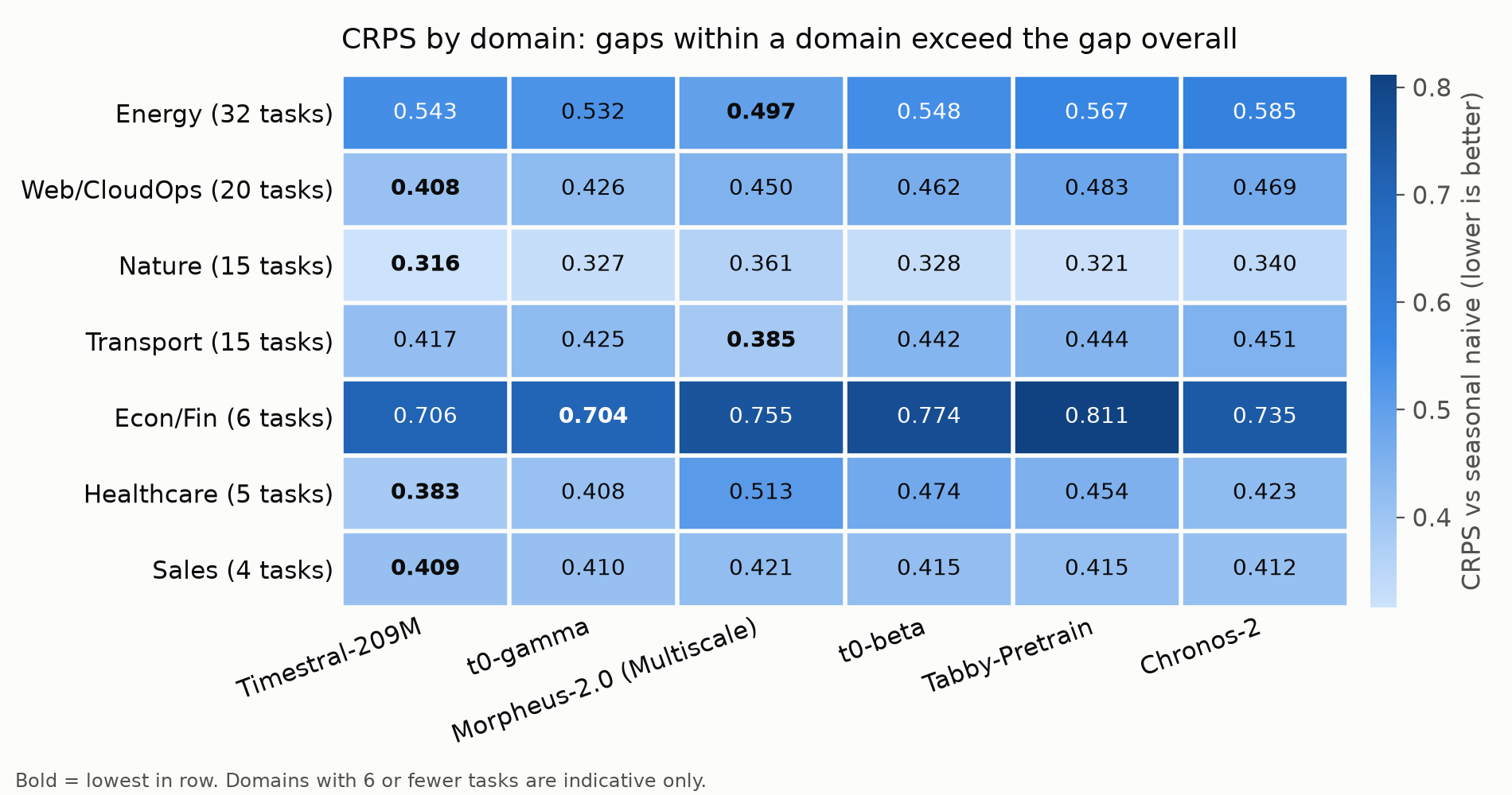
Table 3: Normalised CRPS, geometric mean within each domain. Healthcare, Sales and Econ/Fin contain six or fewer tasks, so their differences are especially uncertain.

Morpheus is about 8% better than Timestral on energy, the largest domain, and also leads on transport. It trails on web, nature and healthcare. Timestral and t0-gamma track each other more closely across domains. One possible explanation is that Morpheus’s every-layer cross-series attention helps on energy and transport datasets containing many correlated meters or sensors. The paper’s own domain table shows similar strengths, but does not isolate attention as the cause.

In the wider heatmap, zero-shot Tabby-Pretrain is second-best on nature despite trailing overall.

Reproducing the three models with public weights

I reran each model with its lab’s own evaluation code: the Timestral notebook in GIFT-Eval, TFC’s t0-gamma notebook and Huawei’s GIFT-Eval script. The only intended changes were the data path and device, plus, for Timestral, halving the batch and retrying when the GPU ran out of memory, which does not change the forecasts. Tabby needed one non-default setting, described below.

I began on an M2 Mac with 24GB of memory, then moved to a single-GPU AWS instance with an NVIDIA A10G and 24GB of memory, costing about $2.45 per hour, after the Mac ran out of memory. Timestral could not use the Mac GPU because its scaling step uses 64-bit floating-point values; on the Mac CPU, the full evaluation would have taken roughly a day. On the A10G, the 97-task t0-gamma ablation took about 90 minutes, and the full t0-gamma rerun about three hours while sharing the GPU with Timestral. Timestral took most of a day, including a restart after it ran out of GPU memory. The instance ran for 22 hours in total and cost about $54.

All three reproduce their official scores. t0-gamma’s CRPS matches to the fourth decimal place and its MASE differs by 0.0001, with every task within 0.25% of the official value. Timestral matches to within one part in a million on every task. Tabby-Pretrain matches exactly, but only with a setting that its evaluation script does not use by default.

With the script’s default settings, Tabby-Pretrain scored 0.4923 CRPS. The median task was identical to the reference, but 15 tasks were more than 5% worse, among them daily COVID deaths (40% worse) and yearly M4 series (31% worse). Tabby’s model card sets --min_forecast_span 128, which makes the masked future at least 128 steps long even when the task asks for fewer; the extra steps are discarded. With that setting every task was within 0.4% of the official value. My guess is that this follows from pretraining, which masks contiguous 128-step blocks: a six-step masked future is unlike anything Tabby learned to fill. If you use Tabby for short horizons, set this option.

What I take from the comparison

The clearest pattern is that recent gains appear to owe a great deal to training data and procedure. Three observations point that way. In Morpheus’s ablations, removing synthetic data and the curriculum costs about 0.13 MASE, compared with about 0.07 when its attention design is replaced by full attention. Tabby’s authors explicitly attribute their gains to data and training. And t0-gamma improves over t0-beta by 0.022 CRPS despite having the same architecture and receiving little help from its inference-time adjustments.

This is an inference from three cases, not a controlled comparison across labs. The strongest alternative explanation is that t0-gamma’s undisclosed training changes made its data more similar to GIFT-Eval, rather than improving general forecasting ability. Testing on series first published after the releases would help distinguish those explanations.

For practitioners, the architectural difference I would investigate first is covariate handling. If demand depends on a known driver such as tomorrow’s temperature, a promotion calendar or scheduled prices, Timestral, t0 and Morpheus can read it; Tabby cannot. GIFT-Eval mostly tests models on their own histories, so its overall leaderboard says relatively little about how effectively they exploit covariates.

Given the aggregate tie, your own data is the better test. A few hundred series from the target domain, evaluated on the actual forecast horizon and covariates you will use, may be more informative than the overall ranking.

Model size also deserves attention. Timestral-28M is only 0.015 CRPS behind Timestral-209M, and Mistral reports about 31 milliseconds per forecast on a CPU. Toto 2.0’s authors likewise recommend a small version as their default. For many production uses, I would start with a smaller model and move up only if a controlled test on my own data showed a meaningful gap.

Licensing can rule out a model before accuracy does. Among these four, t0 is the only one with publicly available weights under Apache-2.0, without the revenue restriction attached to Timestral or Tabby’s non-commercial limitation. Tabby offers unusually complete training code for retraining from scratch (for example, to exclude data you want to reserve for clean evaluation), subject to the same non-commercial weight licence.

The next experiment: energy series with weather covariates

Return to the substation, with its week of hourly load and tomorrow’s temperature forecast. GIFT-Eval does not tell us which of these models forecasts it best when the temperature matters.

The next experiment I would run is a larger collection of energy series paired with real weather forecasts, using test periods beginning after all four releases. I would compare Timestral and t0 with and without their temperature covariate, and use Tabby as a history-only baseline. Morpheus would join once usable public checkpoints are available. I would report both CRPS and MASE, calibration, memory use and wall-clock time, not just an aggregate rank.

That would measure how much accuracy cross-series attention adds when a real covariate is available, and whether the larger models justify their compute on that task.

Code and reproduction materials: tsfm-gifteval-rerun. The code covers pairwise intervals, domain breakdowns, figures and reruns.

Disclaimer:This was an informal, curiosity-driven project undertaken in my personal time. The views expressed here are my own and do not represent those of my employer or any affiliated organisation. The content is based on personal experience and reflection, and should not be taken as professional or academic advice.

📚References

• Mistral AI. (2026, 15 October). Introducing Timestral. Describes the model family’s architecture, synthetic-heavy training, covariate support and CPU performance.

• Meyer, L., et al. (2026). t₀: A Time-Series Foundation Model for Forecasting with Context. Explains the t0 family’s alternating time and cross-series attention, covariate handling and probabilistic forecasts.

• Xie, S., et al. (2026). Tabby: An Open Pretraining Recipe for Time Series Foundation Models. Details channel-independent forecasting, synthetic training data and prompt tuning, distinguishing Tabby-Pretrain from the tuned leaderboard entry.

• Aakriti, et al. (2026). Morpheus-2.0: Multiscale Probabilistic Forecasting with Dual-Axis Attention. Presents gated attention across time and variables, curriculum training and the Multiscale ensemble behind the headline benchmark result.

• Salesforce AI Research. (n.d.). GIFT-Eval. Provides the benchmark, evaluation code and official per-task results underlying the article’s rankings, confidence intervals and domain comparisons.